Zero Shot Image Classification with LanceDB and OpenAI's CLIP

Imagine an AI having a conversation in a language it was never explicitly taught or suddenly playing a new game without any practice. In essence, if an AI can handle a task it hasn’t been directly trained for, that’s what we call zero-shot capability.
Zero-Shot classification
There are many state-of-the-art (SOTA) computer vision models that excel at various classification tasks, such as identifying animals, cars, fraud, and products in e-commerce. They can handle almost any image classification job. However, these models are often specialized and need fine-tuning for different use cases to be truly effective.
Fine-tuning can be challenging; it requires a well-labeled dataset, and if your use case is specific to an enterprise, it may also need significant computing power.
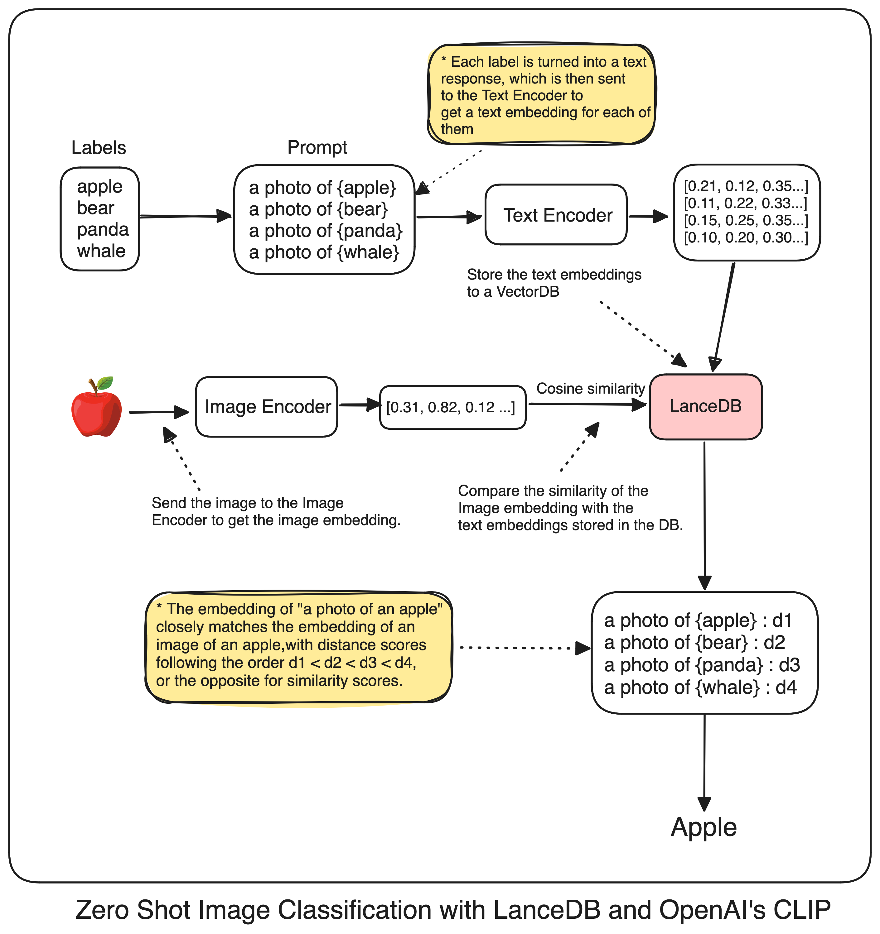
So, what does “Zero-Shot image classification” really means? Imagine a deep learning model trained only to distinguish between cats and dogs. Now, if you show it a picture of a person lounging on the couch playing video games, and the model identifies it as a “corporate employee enjoying a Sunday afternoon,” that’s zero-shot image classification. It means the model can correctly identify something it was never specifically trained to recognize. To help you follow along, here is the complete architecture..
Fundamentals
To make this work, we need a multimodal embedding model and a vector database. Let’s start with something called CLIP, which stands for Contrastive Language-Image Pre-Training. Think of CLIP as a smart box that can understand different types of files. Whether you give it an image or text, it can grasp the context behind them all.
But how it’s working behind the scenes? Consider there are two smaller boxes in that box: a Text Encoder and an Image Encoder. When OpenAI trained CLIP, they made sure these two encoders understand text and images in the same vector space.
They achieved this by training the model to place similar image-text pairs close together in vector space while separating the vectors of non-pairs. Although OpenAI hasn’t specified the exact data used, the CLIP paper mentions that the model was trained on 400 million image-text pairs collected from the internet. This extensive training gives the model an impressive ability to understand relevant image-text pairs.
So, here’s what we get from using CLIP:
- Instead of datasets with specific class labels, CLIP only needs image-text pairs, where the text describes the image.
- Instead of training a CNN to get features from an image, CLIP uses more expressive text descriptions, which can provide additional features.
The authors of CLIP demonstrated its superior zero-shot classification performance by comparing it to the ResNet-101 model trained specifically on ImageNet. When both models were tested on other datasets derived from ImageNet, CLIP outperformed the state-of-the-art ResNet-101, showing a better understanding of the dataset than the fine-tuned version of ResNet-101 trained on ImageNet data.

Reasoning of CLIP
So, the implementation is quite straightforward. But before going into that, Let’s just quickly understand how a CNN works.
Initially, each image in a traditional classification model has assigned class labels. We input these images into the model along with their respective class labels as the expected outputs. Through training, the model’s weights are adjusted based on calculated losses. Over time, the model learns to distinguish between various images by recognizing distinct features.
However, zero-shot classification takes this concept further by utilizing two key components: a Text Encoder and an Image Encoder. Yes those two small boxes that I described earlier, Now these encoders produce n-dimensional vectors for both images and text, mapping them to the same vector space. This means the n-dimensional vector of an image of a “cat” would be semantically similar to the vector of a text description like “a photo of a cat”.
By leveraging this shared vector space, zero-shot classification enables the model to classify images into categories it hasn’t explicitly seen during training. Instead of relying solely on predefined class labels, the model can compare the vector representation of a new image to vector representations of textual descriptions of various categories.

To enhance the effectiveness of our zero-shot classification, we should transform our class labels from simple words like “cat,” “dog,” and “horse” into more descriptive phrases such as “a photo of a cat,” “a photo of a dog,” or “a photo of a horse.” This transformation is crucial because it mirrors the text-image pairs used during the model’s pretraining phase. OpenAI used prompts like "a photo of a {label}" paired with each label to create these image-text pairs.[1]
By adopting a similar approach, our classification task aligns more closely with the model’s pretrained understanding of how images relate to their textual descriptions.
Final thoughts
Let’s take a step back and solidify our understanding before implementation. The CLIP model is pre-trained on a massive dataset of image-text pairs, learning that “a photo of a cat” corresponds to an actual image of a cat, and vice versa. This means whenever we feed an image or text into CLIP, we can expect it to grasp the relevance between the two.
Now, if you want to get into the nitty-gritty of the algorithm, it’s not overly complex. At its core, CLIP encodes each image and text as a n-dimensional embedding vector. Let’s say T1 is the vector for “a photo of a cat”, T2 for “a photo of a bird”, and T3 for “a photo of a horse”. If we have an image of a cat with embedding V1, the similarity score between V1 and T1 should be the highest among all text embeddings. This high similarity tells us that the V1 vector indeed represents “a photo of a cat”.
So, when we pass an image of a cat to our CLIP model, it should reason like “this is a cat, I know this already”. Or if we input an image of bananas on a table, it might get the nerve and put up something like “I think this image shows bananas placed on a table”. Pretty cool, right?
We’ve achieved our goal of classifying images without explicitly training a model on specific categories. And this is how CLIP does the heavy lifting for us, leveraging its pre-training to generalize to a wide range of concepts and enable zero-shot classification.
Using LanceDB
To bring our zero-shot classification system to life, we need a robust Vector Database to store our label embeddings. The process is straightforward: we’ll transform our simple text labels like “cat” into more descriptive phrases such as “a photo of a cat”, fetch their CLIP embeddings, and store these in our database. When it comes time to classify a new image, we’ll retrieve its embedding from CLIP and perform a cosine similarity calculation against all our stored label embeddings in our DB. The label with the closest match becomes our predicted class.
For this crucial task, I’ve opted for LanceDB, an impressive open-source vector database that’s like a super-smart data lake for managing complex information. LanceDB shines when we are handling complex data like our vector embeddings with an exceptional performance in fetching and storage, and the best part? It won’t cost you a dime.
But LanceDB’s appeal goes beyond just being free and open-source. Its unparalleled scalability, efficient on-disk storage, and serverless capabilities make it a standout choice. These features are part of a broader trend of columnar databases that are rapidly transforming ML workflows. I’ve actually written an in-depth article exploring the game-changing capabilities of these kind of databases. If you’re curious about how they’re revolutionizing the field, I highly recommend giving it a read!
Implementation
With all the tools at our disposal, let’s move on to a practical example of using CLIP for zero-shot image classification with the LanceDB vector database. For this demonstration, I’ll use the uoft-cs/cifar100 dataset from Hugging Face Datasets.
from datasets import load_dataset

imagedata = load_dataset(
    'uoft-cs/cifar100',
    split="test"
)

imagedata
Let’s see original label names
# labels names
labels = imagedata.info.features['fine_label'].names
print(len(labels))
labels
100

['apple',
 'aquarium_fish',
 'baby',
 'bear',
 'beaver',
 'bed',
 'bee',
 'beetle',
 'bicycle',
 'bottle',
 'bowl',
 'boy',
 'bridge',
 'bus',
 'butterfly',
 'camel',
 'can',
 'castle',
 'caterpillar',
 'cattle',
 'chair',
 'chimpanzee',
 'clock',
 'cloud',
 'cockroach',
...
 'whale',
 'willow_tree',
 'wolf',
 'woman',
 'worm']
Looks good! We have 100 classes to classify images from, which would require a lot of computing power if you go for traditional CNN. However, let’s proceed with our zero-shot image classification approach.
Let’s generate the relevant textual descriptions for our labels
# generate sentences
clip_labels = [f"a photo of a {label}" for label in labels]
clip_labels
['a photo of a apple',
 'a photo of a aquarium_fish',
 'a photo of a baby',
 'a photo of a bear',
 'a photo of a beaver',
 'a photo of a bed',
 'a photo of a bee',
 'a photo of a beetle',
 'a photo of a bicycle',
 'a photo of a bottle',
 'a photo of a bowl',
 'a photo of a boy',
 'a photo of a bridge',
 'a photo of a bus',
 'a photo of a butterfly',
 'a photo of a camel',
 'a photo of a can',
 'a photo of a castle',
 'a photo of a caterpillar',
 'a photo of a cattle',
 'a photo of a chair',
 'a photo of a chimpanzee',
 'a photo of a clock',
 'a photo of a cloud',
 'a photo of a cockroach',
...
 'a photo of a whale',
 'a photo of a willow_tree',
 'a photo of a wolf',
 'a photo of a woman',
 'a photo of a worm']
Now let’s initialize our CLIP embedding model, I will use the CLIP implementation from hugginface.
# initialization
from transformers import CLIPProcessor, CLIPModel

model_id = "openai/clip-vit-large-patch14"

processor = CLIPProcessor.from_pretrained(model_id)
model = CLIPModel.from_pretrained(model_id)
import torch

# if you have CUDA set it to the active device like this
device = "cuda" if torch.cuda.is_available() else "cpu"
# move the model to the device
model.to(device)
If you’re new to Transformers, remember that computers understand numbers, not text. We’ll convert our text descriptions into integer representations called input IDs, where each number stands for a word or subword, more formally tokens. We’ll also need an attention mask to help the transformer focus on relevant parts of the input.
For more details, you can read about transformers here.
# create label tokens
label_tokens = processor(
    text=clip_labels,
    padding=True,
    return_tensors='pt'
).to(device)

# Print the label tokens with the corresponding text
for i in range(5):
    token_ids = label_tokens['input_ids'][i]
    print(f"Token ID : {token_ids}, Text : {processor.decode(token_ids, skip_special_tokens=False)}")
Token ID : tensor([49406,   320,  1125,   539,   320,  3055, 49407, 49407, 49407]), Text : <|startoftext|>a photo of a apple <|endoftext|><|endoftext|><|endoftext|>
Token ID : tensor([49406,   320,  1125,   539,   320, 16814,   318,  2759, 49407]), Text : <|startoftext|>a photo of a aquarium _ fish <|endoftext|>
Token ID : tensor([49406,   320,  1125,   539,   320,  1794, 49407, 49407, 49407]), Text : <|startoftext|>a photo of a baby <|endoftext|><|endoftext|><|endoftext|>
Token ID : tensor([49406,   320,  1125,   539,   320,  4298, 49407, 49407, 49407]), Text : <|startoftext|>a photo of a bear <|endoftext|><|endoftext|><|endoftext|>
Token ID : tensor([49406,   320,  1125,   539,   320, 22874, 49407, 49407, 49407]), Text : <|startoftext|>a photo of a beaver <|endoftext|><|endoftext|><|endoftext|>
Now let’s get our CLIP embeddings for our text labels
# encode tokens to sentence embeddings from CLIP

with torch.no_grad():
    label_emb = model.get_text_features(**label_tokens) # passing the label text as in "a photo of a cat" to get it's relevant embedding from clip model

# Move embeddings to CPU and convert to numpy array
label_emb = label_emb.detach().cpu().numpy()
label_emb.shape
(100, 768)
We now have a 768-dimensional vector for each of our 100 text class sentences. However, to improve our results when calculating similarities, we need to normalize these embeddings.
Normalization helps ensure that all vectors are on the same scale, preventing longer vectors from dominating the similarity calculations simply due to their magnitude. We achieve this by dividing each vector by the square root of the sum of the squares of its elements. This process, known as L2 normalization, adjusts the length of our vectors while preserving their directional information, making our similarity comparisons more accurate and reliable.
import numpy as np

# normalization
label_emb = label_emb / np.linalg.norm(label_emb, axis=0)
label_emb.min(), label_emb.max()
Ok, let’s see a random image from our dataset
import random

index = random.randint(0, len(imagedata)-1)
selected_image = imagedata[index]['img']
selected_image
When you execute this code, you’ll be presented with a visual representation of a data point from our dataset. In my case, the output displayed a pixelated image of a whale.

Before we can analyze our image with CLIP, we need to preprocess it properly. First, we’ll run the image through our CLIP processor. This step ensures the image is resized first, then the pixels are normalized, then converting it into the tensor and finally adding a batch dimension. All of these things are settled up for the model.
image = processor(
    text=None,
    images=imagedata[index]['img'],
    return_tensors='pt'
)['pixel_values'].to(device)
image.shape
torch.Size([1, 3, 224, 224])
Now here this shape represents a 4-dimensional tensor:
- 1: Batch size (1 image in this case)
- 3: Number of color channels (Red, Green, Blue)
- 224: Height of the image in pixels
- 224: Width of the image in pixels
So, we have one image, with 3 color channels, and dimensions of 224x224 pixels. Now we’ll use CLIP to generate an embedding - a numerical representation of our image’s features. This embedding is what we’ll use for our classification task.
img_emb = model.get_image_features(image)
img_emb.shape
torch.Size([1, 768])
This gives us 768 dimensional embedding to us, that’s our Image Embedding. Only thing that is left for now is to use LanceDB to store our labels, with their corresponding embeddings and do the vector search for our Image Embedding on that database.. Here how it looks in the whole go
import lancedb
import numpy as np

data = []
for label_name, embedding in zip(labels, label_emb):
    data.append({"label": label_name, "vector": embedding})

db = lancedb.connect("./.lancedb")
table = db.create_table("zero_shot_table", data, mode="Overwrite")

# Prepare the query embedding
query_embedding = img_emb.squeeze().detach().cpu().numpy()
# Perform the search
results = (table.search(query_embedding)
           .limit(10)
           .to_pandas())

print(results.head(n=10))
|   label         | vector | distance |
|-----------------|-----------------------------------------------------------|-------------|
| whale           | [0.05180167, 0.008572296, -0.00027403078, -0.12351207, ...]| 447.551605  |
| dolphin         | [0.09493398, 0.02598409, 0.0057568997, -0.13548125, ...]| 451.570709  |
| aquarium_fish   | [-0.094619915, 0.13643932, 0.030785343, 0.12217164, ...]| 451.694672  |
| skunk           | [0.1975818, -0.04034014, 0.023241673, 0.03933424, ...]| 452.987640  |
| crab            | [0.05123004, 0.0696855, 0.016390173, -0.02554354, ...]| 454.392456  |
| chimpanzee      | [0.04187969, 0.0196794, -0.038968336, 0.10017315, ...]| 454.870697  |
| ray             | [0.10485967, 0.023477506, 0.06709562, -0.08323726, ...]| 454.880524  |
| sea             | [-0.08117988, 0.059666794, 0.09419422, -0.18542227, ...]| 454.975311  |
| shark           | [-0.01027703, -0.06132377, 0.060097754, -0.2388756, ...]| 455.291901  |
| keyboard        | [-0.18453166, 0.05200073, 0.07468183, -0.08227961, ...]| 455.424866  |
Here are the results everyone: all set and confirmed. Our initial accurate prediction is a whale, demonstrating the closest resemblance between the label and the image with minimal distance, just as we had hoped. What’s truly remarkable is that we achieved this without running a single epoch for a CNN model. That’s zero shot classification for you fellas. Here is your colab for your reference. See you in next one.